이번 글은 cs231n 3강에서 다뤘던 수식이나 알고리즘을 직접 파이썬으로 구현해서 작성했다.
✍️ SVM Loss

# simple loss function

# 0 : cat, 1 : car, 2 : frog
def SVM_loss(score):
    result = 0

    for i in range(3):
        for j in range(len(score)):
            if i == j:
                continue
            else:
                result += max(0,score[i][j] - score[i][i] + 1)
        print(result)

    return result // 3


score = [[3.2,5.1,-1.7],[1.3,4.9,2.0],[2.2,2.5,-3.1]]

print(SVM_loss(score))- 위 코드는 SVM loss의 수식을 간단하게 파이썬으로 구현한 결과이다.
- 3으로 하드코딩된 곳은 Lable의 개수에 따라 변경해야한다.
✍️ Softmax Loss
# simple Softmax Function
# 0 : cat, 1 : car, 2 : frog
import numpy as np

def softmax(score):
    loss_list = []
    for i in range(len(score)):
        exp_score = np.exp(score[i])

        for j in range(len(exp_score)):
            eyi = exp_score[j]
            sum_esj = sum(exp_score)
            loss_list.append(-np.log10(eyi/sum_esj))

    return loss_list


score = np.array([[3.2,5.1,-1.7],[1.3,4.9,2.0],[2.2,2.5,-3.1]])
print(softmax(score))- 위 코드는 Softmax Loss를 간단하게 파이썬으로 구현하였다. 숫자는 위 사진의 예시에 따라 작성하였다.
- 지수의 승으로 표현해주고, Normalize를 해주는 것이 핵심
✍️ Gradient Descent
- Gradient Descent (경사 하강법)은 적절한 가중치를 찾는데 사용되며, 기본 원리는 -gradient 방향으로 진행하며 기울기가 0인 지점을 찾는 것이 목표이다.
import numpy as np
import matplotlib.pyplot as plt

def example_function(x):
    return (x**2)

def gradient(x):
    df = 2*x
    return df

def gradient_descent(init_x, learning_rate, epoch):
    x = init_x
    x_history = [x]

    for i in range(epoch):
        grad = gradient(x)
        x = x - learning_rate * grad
        x_history.append(x)

    return x_history

init_x = -4.5
learning_rate = 0.01
epoch = 100

x_history = gradient_descent(init_x, learning_rate, epoch)

x = np.arange(-5,5,0.01)
y = example_function(x)

plt.plot(x,y)
plt.plot(x_history, [example_function(x) for x in x_history], 'ro-')
plt.show()- 위 코드는 x^2 함수에서의 경사하강법을 시각화한 코드이다. init_x에서 learning_rate만큼 하강하며 0인 지점에서 x의 변화가 멈추게 된다.
- 위 사진은 learning_rate가 0.01일 경우이다. 사진에서는 완벽하게 기울기가 0인 지점으로 가지 못했는데, 이는 epoch(반복횟수)를 늘려주면 해결된다. 발산 없이 잘 찾아가는 것을 볼 수 있다.
- 위 사진은 learning_rate 0.8, epoch 1000일 경우인데 발산하며 왔다갔다 하다가 0을 찾아가는 것을 볼 수 있다. learning_rate가 더 늘어나면 아마 엉뚱한 곳에 위치할 것이다.
✍️ Numerical Gradient
- Numerical Gradient는 f(x+h)-f(x) / h 의 식을 이용해서 경사하강법을 적용하는 방식이다. 느리지만 정확하여 디버깅에 사용된다고한다.
import numpy as np

# 초기값들
init_W = [[0.2,-0.5,0.1,2.0], [1.5,1.3,2.1,0.0],[0,0.25,0.2,-0.3]]
init_b = [1.0,1.0,1.0]
w = np.array(init_W).reshape((3,4))
b = np.array(init_b).reshape((3,1))
lr = 0.0001

#svm loss를 구현, margin이 1e-8인 이유는 1로 하니 너무 쉽게 발산되어 더 작은 수로 설정하였다.
def SVM_loss(score):
    result = 0

    for i in range(len(score)):
        for j in range(len(score)):
            if i==j:
                continue
            else:
                result += max(0,score[j]-score[i]+1e-8)
    return result / len(score)

# linear classification
def f(w):
    global b
    w = w.reshape(3,4)
    x = [56,23,24,2]
    x = np.array(x).reshape(4,1)
    return (w @ x) + b

# numerical gradient를 통한 경사하강법 구현 f(w+h) - f(w) / h
def numerical_gradient(w):
    w =  w.flatten()
    h = 0.01
    w_plus = w.copy()

    grad = np.zeros_like(w)
    for i in range(len(w)):
        w_plus[i] += h
        grad[i]= (SVM_loss(f(w_plus)) - SVM_loss(f(w))) / h

    return grad

# 가중치를 gradient 반대로 증가 learning rate 곱해줌
def update_weight(w):
    dw = numerical_gradient(w)
    dw = dw.reshape(3,4)
    w += - lr*dw
    return w

# epoch : 1000
for i in range(1001):
    score = f(w)
    if i % 100 == 0:
        print("epoch : ",i,"loss: ",SVM_loss(score))
w = update_weight(w)- 일단 예시의 숫자, size를 어느정도 따와서 구현하였다. 은근히 구현이 버거웠으며, 아직 행렬을 다루는데 익숙치 않은 것 같다..
- lr가 0.01 이였는데, 이때 너무 빠르게 발산이 일어났다. 그래서 lr을 줄이고 epoch도 늘렸더니 loss가 0까지 도달은 했다. 하이퍼파라미터 조절이 굉장히 중요하다는 것을 느낄 수 있었다.
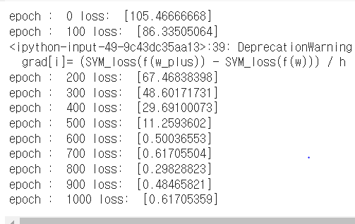
- 위 코드의 실행결과인데 loss가 0에 가까워짐을 볼 수 있다. 내 코드가 맞는지 모르겠지만, 일단 loss가 줄어드는 쪽으로 작동한다.
- analystic gradient는 다음장에서 chain rule을 배우고 구현할 예정이다.
✍️ Reference
'AI > algorithm' 카테고리의 다른 글
| [Algorithm] L1, L2, NN, KNN, Linear Classifier (2) | 2024.02.28 |
|---|
